Saprophytic fitness
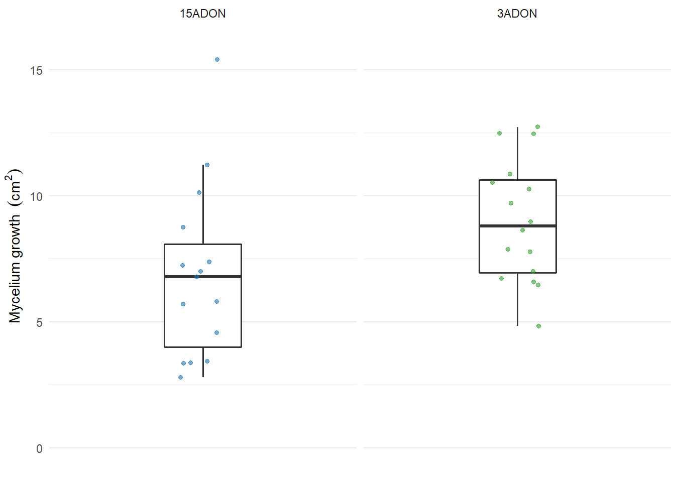
Mycelium growth
mycelium <- read_excel("data/dat-fitness.xlsx", sheet = "mycelium")

# Removing the mycelium plug area
mycelium["day1"] = mycelium["d1_cm"] -0.283
mycelium["day2"] = mycelium["d2_cm"] -0.283


# Estimating the average radial growth rate (cm2 per day)
mycelium$growth <- (mycelium$day2 - mycelium$day1)


# Summarizing the data
mycelium1 <- mycelium %>%
  group_by(experiment, isolate, tri, rep) %>% summarize(mgr = mean(growth))


plot_mycelium <- mycelium1 %>%
  group_by(isolate, tri) %>%
  summarise(growth = mean(mgr, na.rm = T)) %>%
  ggplot(aes(tri, growth))+
  geom_boxplot(size = 0.6,
               outlier.colour = NA, width=0.3
               ) +
  geom_jitter(size = 1.3, width = 0.1,
              alpha=0.6, aes(color=tri))+
    facet_grid (~ tri, scales = "free") +
  theme_minimal()+
  scale_color_manual(breaks = c("15ADON", "3ADON"),  values=c("#1F78B4", "#33A02C"))+
  scale_fill_manual(breaks = c("15ADON", "3ADON"),  values=c("white", "white"))+
  theme(legend.position = "none",
        plot.margin = unit(c(-0.6, 0.1, -0.2, 0.1), "cm"),
        legend.margin=margin(0,0,0,0),
        legend.box.margin=margin(-0,-10,-10,-10),
        panel.grid.major.x = element_blank(),
        axis.text.x=element_blank())+
labs(y = expression(paste("Mycelium growth " ~ (cm^2))),
                      x = "",
                      title = "",
      color = "", fill = "")+
  ylim(0, 16)

plot_mycelium
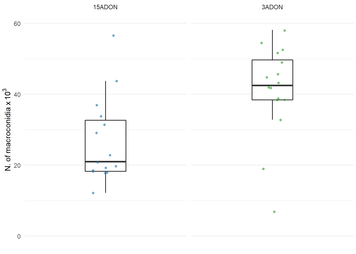
Macroconidia production
conidia <- read_excel("data/dat-fitness.xlsx", sheet = "conidia")

conidia1 <- conidia %>%
  group_by(experiment, isolate, tri, rep) %>% summarize(spores = mean(conc_spores))


plot_conidia <- conidia1 %>%
  group_by(isolate, tri) %>%
  summarise(conidia = mean(spores, na.rm = T)) %>%
  ggplot(aes(tri, conidia)) +
  geom_boxplot(size = 0.6,
               outlier.colour = NA, width=0.3
               ) +
  geom_jitter(size = 1.3, width = 0.1,
              alpha=0.6, aes(color=tri)) +
  facet_grid (~ tri, scales = "free") +
  theme_minimal() +
  scale_color_manual(breaks = c("15ADON", "3ADON"),  values=c("#1F78B4", "#33A02C")) +
  scale_fill_manual(breaks = c("15ADON", "3ADON"),  values=c("white", "white")) +
  theme(legend.position = "none",
        plot.margin = unit(c(-0.6, 0.1, -0.2, 0.1), "cm"),
        legend.margin=margin(0,0,0,0),
        legend.box.margin=margin(-0,-10,-10,-10),
        panel.grid.major.x = element_blank(),
        axis.text.x=element_blank())+
labs(y = expression(N.~of~macroconidia~x~10 ^ {3}),
      x = "", title = "",
      color = "", fill = "")+
  ylim(0,60)

plot_conidia
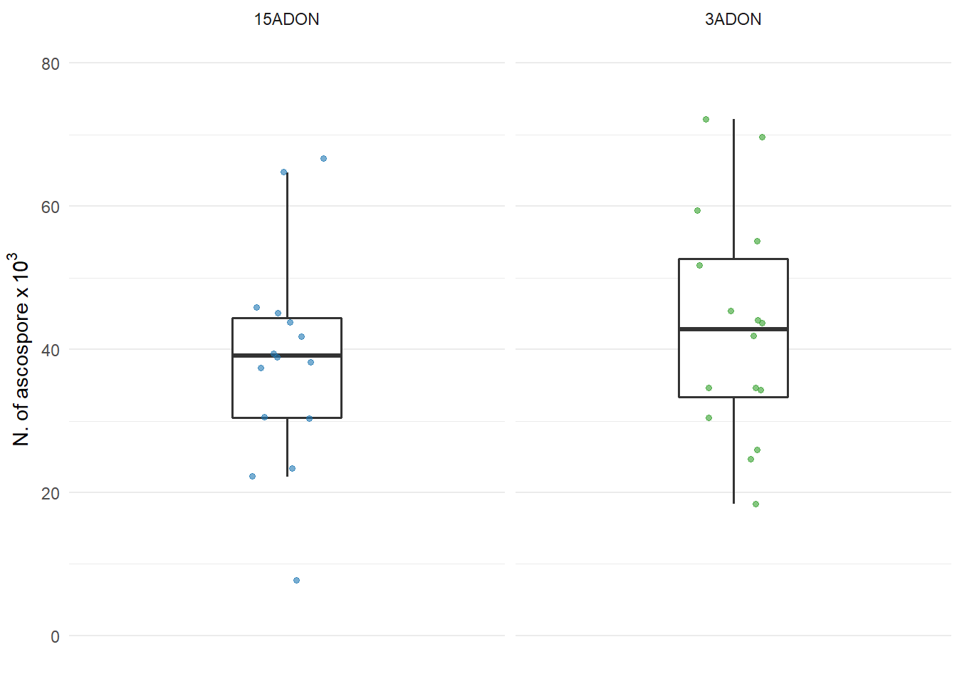
Ascospore production
ascospore <- read_excel("data/dat-fitness.xlsx", sheet = "ascospore")

ascospore1 <- ascospore %>%
  group_by(experiment, isolate, tri, location, region, crop, rep) %>% summarize(ascospore = mean(conc_spores))

plot_ascospore <- ascospore1 %>%
  group_by(isolate, tri) %>%
  summarise(ascospore = mean(ascospore, na.rm = T)) %>%
  ggplot(aes(tri, ascospore)) +
  geom_boxplot(size = 0.6,
               outlier.colour = NA, width=0.3,
               #position = position_dodge(width = 0.9)
               ) +
  geom_jitter(size = 1.3, width = 0.1,
              #position=position_jitterdodge(dodge.width=0.9),
              alpha=0.6, aes(color=tri))+
  #scale_fill_grey(start = 1, end = 1)+
  facet_grid (~ tri, scales = "free") +
  theme_minimal()+
  scale_color_manual(breaks = c("15ADON", "3ADON"),  values=c("#1F78B4", "#33A02C"))+
  scale_fill_manual(breaks = c("15ADON", "3ADON"),  values=c("white", "white"))+
  theme(legend.position = "none",
        plot.margin = unit(c(-0.6, 0.1, -0.2, 0.1), "cm"),
        legend.margin=margin(0,0,0,0),
        legend.box.margin=margin(-0,-10,-10,-10),
        panel.grid.major.x = element_blank(),
        axis.text.x=element_blank())+
labs(y = expression(N.~of~ascospore~x~10 ^ {3}),
      x = "", title = "",
      color = "", fill = "")+
  ylim(0,80)

plot_ascospore
Perithecia production
peritecia <- read_excel("data/dat-fitness.xlsx", sheet = "perithecia")

peritecia1 = peritecia %>%
  gather("Day 3", "Day 6", key = day, value = percentage) %>%
  arrange(isolate)

plot_perithecia <- peritecia1 %>%
  group_by(isolate, tri, day) %>%
  summarise(percentage = mean(percentage, na.rm = T)) %>%
  ggplot(aes(x = day,
             y = percentage,
             fill = tri)) +
  geom_boxplot(size = 0.6,
               outlier.colour = NA, width=0.3,
               position = position_dodge(width = 0.5)
               ) +
  geom_jitter(position=position_jitterdodge(dodge.width=0.5, jitter.width = 0.1),
              size=1.3,
              alpha=0.6,
              aes(colour=tri)) +
  theme_minimal() +
  scale_color_manual(breaks = c("15ADON", "3ADON"), values=c("#1F78B4", "#33A02C"))+
  scale_fill_manual(breaks = c("15ADON", "3ADON"), values=c("white", "white")) +
  labs(y = expression(paste("Perithecia production (%)")),
                      x = "",
                      title = "",
      color = "", fill = "") +
  theme(legend.position = "top",
        plot.margin = unit(c(-0.6, 0.1, -0.2, 0.1), "cm"),
        legend.margin=margin(0,0,0,0),
        legend.box.margin=margin(-0,-10,-10,-10),
        panel.grid.major.x = element_blank())

plot_perithecia
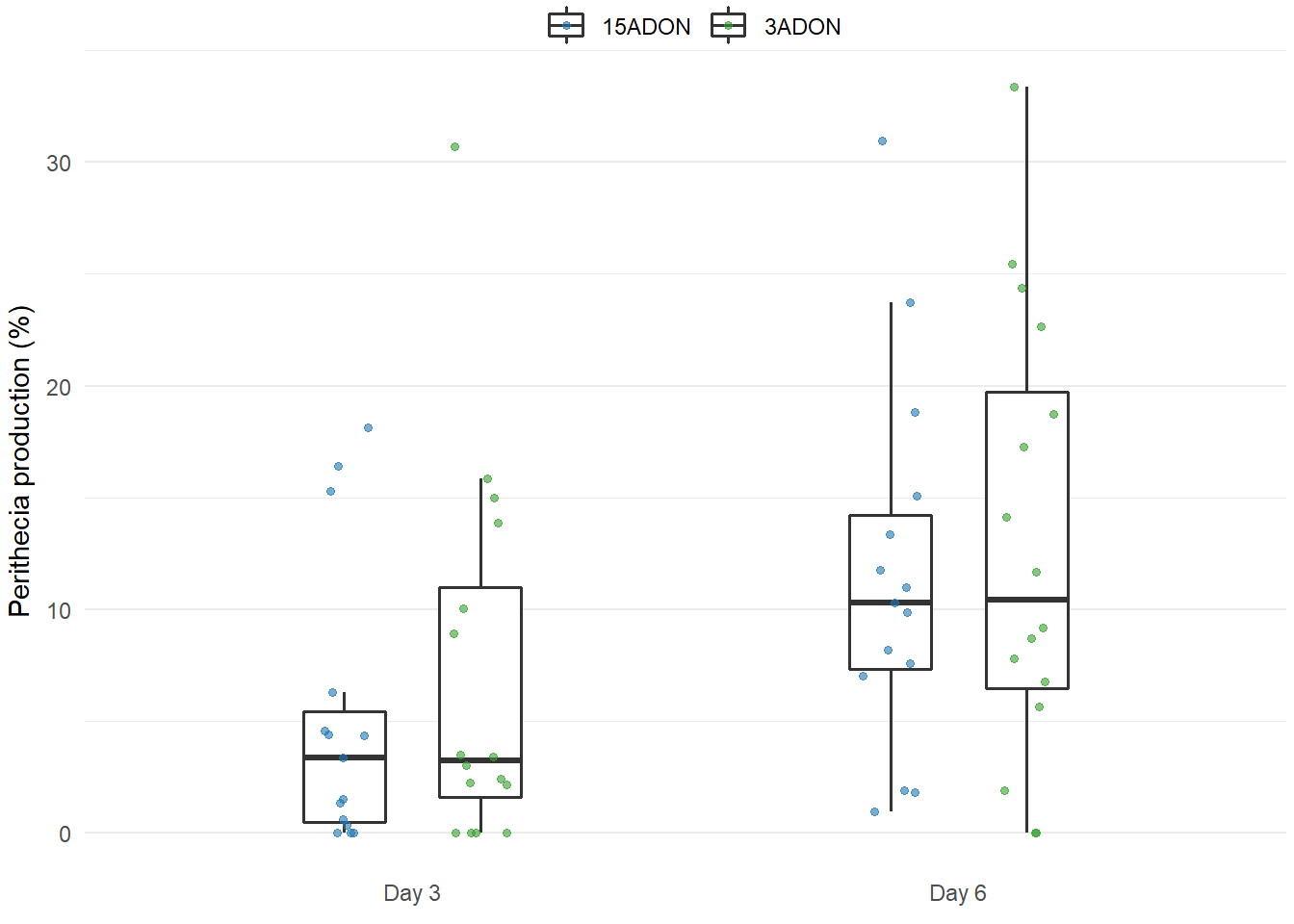
FIG 1 - GRID
grid1 <- plot_grid(plot_mycelium, plot_conidia, plot_ascospore, plot_perithecia, labels=c('A', 'B', 'C', 'D'), align = "hv", ncol=2) +

ggsave("figures/grid1.png",  width=10, height=5, dpi=300)

grid1
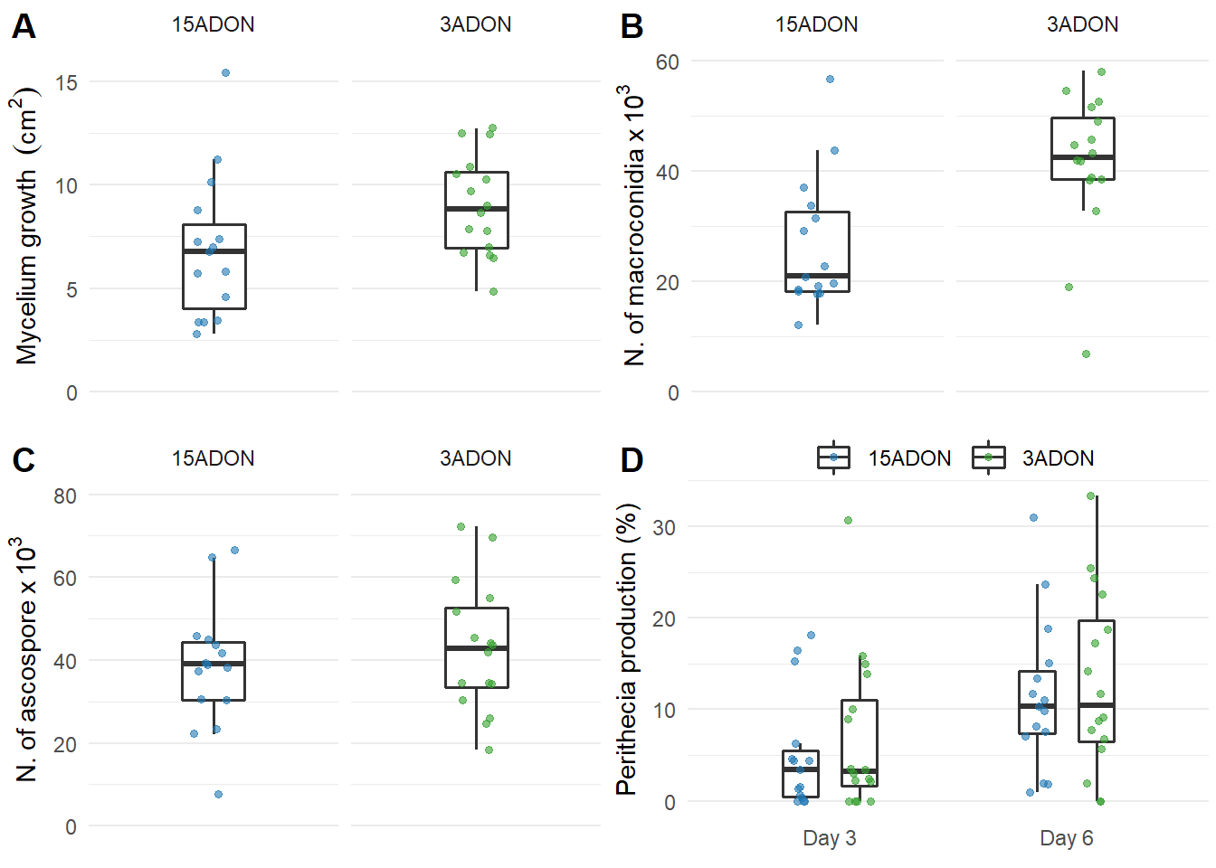
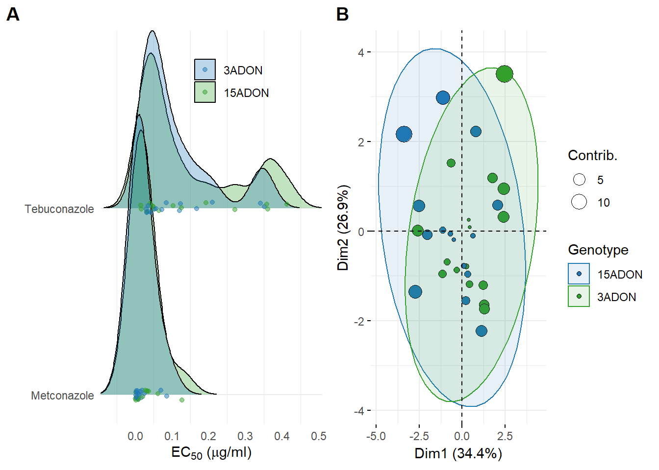
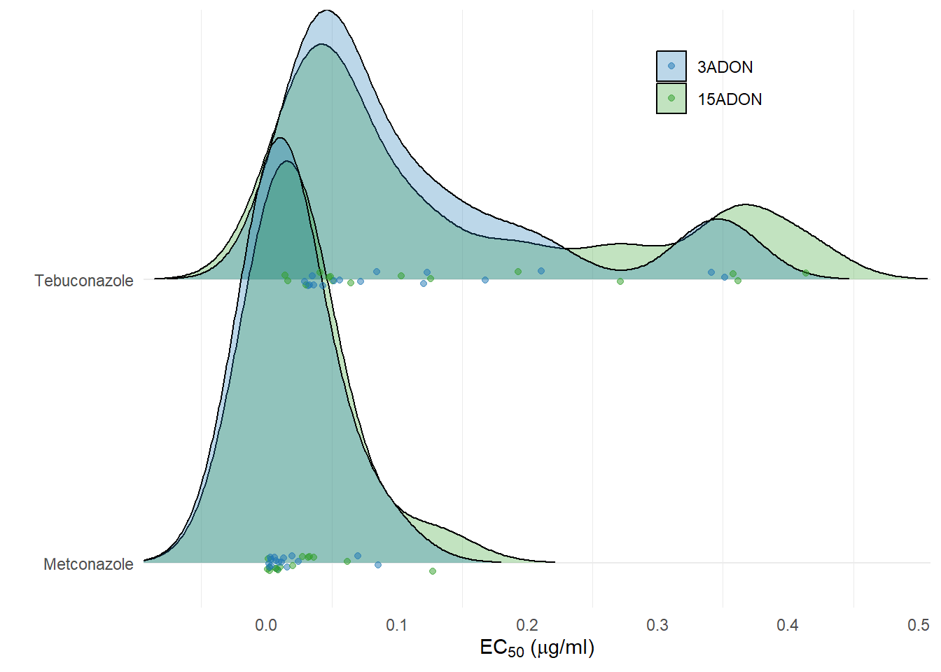
FIG 2 - EC50 and PCA
Fungicide
fung <- read_csv("data/ec50.csv")

ec50 <- fung %>%
  select(-X1)

plot_fungicide <- ec50 %>%
  group_by(isolate, tri, fungicide) %>%
  summarise(ec50 = mean(Estimate, na.rm = T)) %>%
  ggplot(aes(x = ec50, fungicide,  fill = factor(tri))) +
  geom_joy(scale = 1.5, alpha = 0.3, rel_min_height = 0.001) +
  geom_jitter(alpha=0.5, height = 0.03, size = 1.5, aes(color = factor(tri)))  +
  scale_color_manual(breaks = c("3ADON", "15ADON"),  values =  c(alpha("#1F78B4", 0.5), alpha("#33A02C", 0.5))) +
  scale_fill_manual(breaks = c("3ADON", "15ADON"), values = c(alpha("#1F78B4", 0.5), alpha("#33A02C", 0.5))) +
  scale_y_discrete(expand = c(0.01, 0.15)) +
  scale_x_continuous(expand = c(0, 0)) +
  theme_minimal() +
  theme(legend.position = c(0.8, 1),
        #plot.margin = unit(c(0, 0.1, -0.2, 0.1), "cm"),
        legend.justification = c("right", "top"),
        panel.grid.major.x = element_blank(),
        axis.title.x = element_text(hjust=0.5))+
  labs(x = (expression(paste('EC'[50], ' (', mu,'g/ml)'))), y = "", fill = "", color = "")

plot_fungicide
PCA analysis
dat_multivar <- read_csv("data/dat_multivar.csv") %>%
  select(-isolate) %>%
  select(-X1)

dat_mul_new <- dat_multivar %>%
  rename(Genotype = tri)


# Selecting only the dependent variables

dat_multivar_pca <- dat_multivar %>%
  select(-tri)

res.pca <- PCA(dat_multivar_pca, graph = FALSE)


## Graphic

biplot <- fviz_pca_biplot(res.pca,
                geom.ind = "point",
                fill.ind = dat_mul_new$Genotype, #col.ind = "black",
                pointshape = 21,
                pointsize = "contrib",
                mean.point = FALSE, #remove group mean point
                palette = c("#1F78B4", "#33A02C"),
                addEllipses = TRUE, #ellipse.type = "confidence",ellipse.level = 0.95,
                # Variables
                alpha.var ="contrib",
                invisible = "var",
                )+
  scale_color_manual( values=c("#1F78B4", "#33A02C")) +
  labs(title = "", fill = "Genotype", color = "Genotype", size = "Contrib.")


biplot
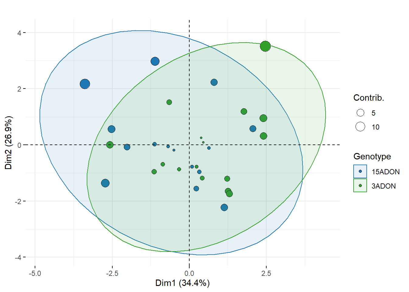
FIG 2 - GRID
grid2 <- plot_grid(plot_fungicide, biplot, labels=c('A', 'B'), align = "hv") +

ggsave("figures/grid2.png", width=10, height=4, dpi=300)
## Picking joint bandwidth of 0.0318
grid2